Introduction to TensorFlow for AI, ML, and DL

I took the Coursera course called Introduction to TensorFlow for Artificial Intelligence, Machine Learning, and Deep Learning taught by Laurence Moroney when attending an Amazon internal guild learning section recently. Here are the notes of what I learnt from the course and also some thoughts that can help you decide whether to take the course.
Week 1
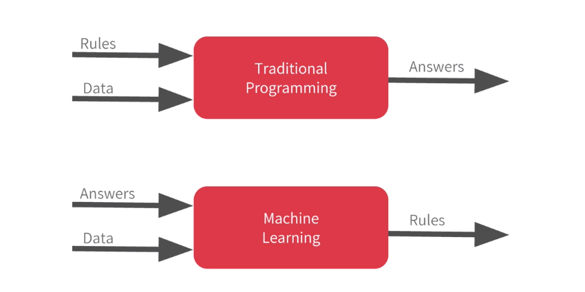
Traditional Programming takes Rule + Data to output Answers, but Machine Learning learns Rules from Answers + Data.
TensorFlow practice: The NN contains a single layer with 1 neuron trained with SDG + MSE after 500 epochs using 6 data points generated by linear function y = 2x - 1 :
from tensorflow import keras
import numpy as np

# Define the model
model = keras.Sequential([keras.layers.Dense(units=1, input_shape=[1])])
model.compile(optimizer='sgd', loss='mean_squared_error')

# Data
xs = np.array([-1.0,  0.0, 1.0, 2.0, 3.0, 4.0], dtype=float)
ys = np.array([-3.0, -1.0, 1.0, 3.0, 5.0, 7.0], dtype=float)

# Train
model.fit(xs, ys, epochs=500)

# Predict
print(model.predict([10.0]))
What is epoch? An epoch is one complete presentation of the data set to be learned to a learning machine. Learning machines like feedforward neural nets that use iterativealgorithms often need many epochs during their learning phase. link
Also, this website, TensorFlow PlayGround, is very interesting to manually adjust NN structure and see the visualized hiddhen layer outputs and generated models. I feel good to have a direct feeling to see how a super large NN can easily overfitting the limited data. --> get more data!!! ;)
Week 2
Train a NN on FashionMnist dataset. This is a 3 layers NN with 1 input layer, 1 hidden layer, and 1 fully connected layer for output. Try the Colab notebook here.
import tensorflow as tf
from tensorflow import keras

# Get Fashion-Mnist
mnist = keras.datasets.fashion_mnist
(train_imgs, train_labels), (test_imgs, test_labels) = mnist.load_data()

# Have a look at the data
import matplotlib.pyplot as plt
plt.imshow(train_imgs[0])
print(train_imgs[0])
print(train_labels[0])

# Normalization
train_imgs  = train_imgs / 255.0
test_imgs = test_imgs / 255.0

# Define the model
model = keras.models.Sequential([keras.layers.Flatten(),
                                 keras.layers.Dense(128, activation=tf.nn.relu, input_shape=(784, 1)),
                                 keras.layers.Dense(10, activation=tf.nn.softmax)])

# Compile model
model.compile(optimizer='adam',
              loss='sparse_categorical_crossentropy',
              metrics=['accuracy'])

# Train model
model.fit(train_imgs, train_labels, epochs=5)

# Test model
import numpy as np
plt.imshow(test_imgs[0])
print(model.predict(np.reshape(test_imgs[0], (1, 28, 28))))

model.evaluate(test_imgs, test_labels)
Qs:
- What will happen when set the hidden layer's neurons number to 512?
- Training time increase, accuracy also increase
- What will happen if you remove the
Flatten()layer?- Throw error, as
(28, 28)input image cannot fit intoinput_shapeof(784, 1)
- Throw error, as
- What will happen if you add two more layers with 256 and 128 neurons?
- No significant impact as this complex NN overfitting the simple data.
- What will happen if you remove the normalization?
- It becomes hard for NN to learn and you'll see big loss in the beginning
- Can we do early stop in TensorFlow to prevent overfitting?
- Yes! See the example using callback below.
import tensorflow as tf

# Define callback function
class myCallback(tf.keras.callbacks.Callback):
  def on_epoch_end(self, epoch, logs={}):
    if(logs.get('acc')>0.80):
      print("\nReached 80% accuracy so cancelling training!")
      self.model.stop_training = True

callbacks = myCallback()
mnist = tf.keras.datasets.fashion_mnist
(training_images, training_labels), (test_images, test_labels) = mnist.load_data()
training_images, test_images = training_images / 255.0, test_images / 255.0
model = tf.keras.models.Sequential([
  tf.keras.layers.Flatten(),
  tf.keras.layers.Dense(512, activation=tf.nn.relu),
  tf.keras.layers.Dense(10, activation=tf.nn.softmax)
])
model.compile(optimizer='adam', loss='sparse_categorical_crossentropy')
model.fit(training_images, training_labels, epochs=5, callbacks=[callbacks])
In addition, this website: ML Faireness by Google is interesting talking about bias in ML.
Week 3
CNN for this week. The instructor introduced the convolution and pooling. They are corresponding to the Conv2D layer and MaxPooling2D layers in tf.keras. For details on how CNN works, check Convolutional Neural Networks (Course 4 of the Deep Learning Specialization)
Notebook for the codes below: Link in Colab or Link in GitHub.
import tensorflow as tf
print(tf.__version__)
mnist = tf.keras.datasets.fashion_mnist
(training_images, training_labels), (test_images, test_labels) = mnist.load_data()
training_images=training_images.reshape(60000, 28, 28, 1)
training_images=training_images / 255.0
test_images = test_images.reshape(10000, 28, 28, 1)
test_images=test_images/255.0
model = tf.keras.models.Sequential([
  tf.keras.layers.Conv2D(64, (3,3), activation='relu', input_shape=(28, 28, 1)),
  tf.keras.layers.MaxPooling2D(2, 2),
  tf.keras.layers.Conv2D(64, (3,3), activation='relu'),
  tf.keras.layers.MaxPooling2D(2,2),
  tf.keras.layers.Flatten(),
  tf.keras.layers.Dense(128, activation='relu'),
  tf.keras.layers.Dense(10, activation='softmax')
])
model.compile(optimizer='adam', loss='sparse_categorical_crossentropy', metrics=['accuracy'])
model.summary()
model.fit(training_images, training_labels, epochs=5)
test_loss = model.evaluate(test_images, test_labels)
Note that for the Conv layer Conv2D(64, (3, 3), activation='relu', input_shape=(28, 28, 1)), 64 means the number of filters (conv kernel), 3 x 3 is the size of conv kernel, and the input shape is 28 x 28 x 1, which represents: width x height x color depth. As all pictures in FashionMNIST are gray level with only one color channel from 1 to 255, the last dimension of the input shape should be 1.
Let's have a close look at the parameters by model.summary():
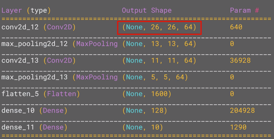
Why does the output after 1st conv layer change from 28x28 to 26x26? Consider: the filter is 3x3 size, and for each time, it moves 1 pixel to the right (called Stride, check the video).
Let's print the feature maps, i.e. visualize the outputs of each layer:
import matplotlib.pyplot as plt
f, axarr = plt.subplots(3,4)
FIRST_IMAGE=0
SECOND_IMAGE=23
THIRD_IMAGE=28
CONVOLUTION_NUMBER = 6
from tensorflow.keras import models
layer_outputs = [layer.output for layer in model.layers]
activation_model = tf.keras.models.Model(inputs = model.input, outputs = layer_outputs)
for x in range(0,4):
  f1 = activation_model.predict(test_images[FIRST_IMAGE].reshape(1, 28, 28, 1))[x]
  axarr[0,x].imshow(f1[0, : , :, CONVOLUTION_NUMBER], cmap='inferno')
  axarr[0,x].grid(False)
  f2 = activation_model.predict(test_images[SECOND_IMAGE].reshape(1, 28, 28, 1))[x]
  axarr[1,x].imshow(f2[0, : , :, CONVOLUTION_NUMBER], cmap='inferno')
  axarr[1,x].grid(False)
  f3 = activation_model.predict(test_images[THIRD_IMAGE].reshape(1, 28, 28, 1))[x]
  axarr[2,x].imshow(f3[0, : , :, CONVOLUTION_NUMBER], cmap='inferno')
  axarr[2,x].grid(False)
The 6th (counting from 0) conv kernel is good at capture the whole shoes:
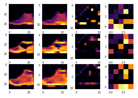
The 9th conv kernel is good at capture the feature of shoe soles:

What's the idea of convolution? Look at this notebook to have a deeper understanding of how does those "filters" find the "features": Link in Colab or Link in GitHub. Some more interesting filters in Lode's Computer Graphics Tutorial.
The definitions of Convolution and Pooling given in the Quiz are very straight forward:
- Convolution: A technique to isolate features in images
- Pooling: A technique to reduce the informaiton in an image while maintaining features
Week 4
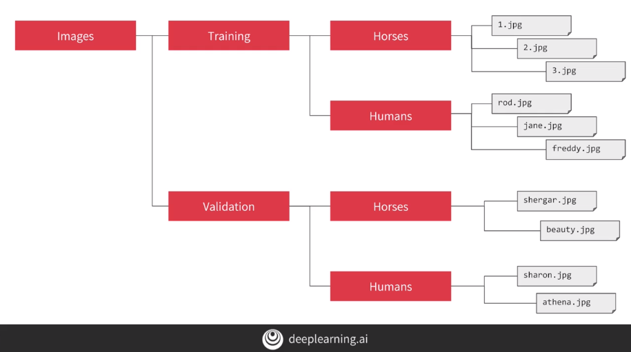
Lets assume we are trying to distinguish horse pictures from human pictures. To get the datasets from directory, we can use ImageGenerator to load the datasets as following:
ImageGenerator codes to do that:
from tensorflow.keras.preprocessing.image import ImageDataGenerator
train_datagen = ImageDataGenerator(rescale=1./255)  // to normalize the data
train_generator = train_datagen.flow_from_directory(
    train_dir,
  target_size=(300, 300),
  batch_size=128,  // pass in 128 images as one batch
  class_mode='binary'
)

validate_datagen = ImageDataGenerator(rescale=1./255)  // to normalize the data
validate_generator = validate_datagen.flow_from_directory(
    validate_dir,
  target_size=(300, 300),
  batch_size=32,  // pass in 32 images as one batch
  class_mode='binary'
)
It's a common mistake to point the train_dir to the sub-directories. You shoud set the train_dir as the parent directory of the sub-directories which each name is reagrded the label of images that are contained within them.
Then define the model:
model = tf.keras.models.Sequential([
  tf.keras.layers.Conv2D(16, (3, 3), activation='relu', input_shape=(300, 300, 3)),
  tf.keras.layers.MaxPooling2D(2, 2),
  tf.keras.layers.Conv2D(32, (3, 3), activation='relu'),
    tf.keras.layers.MaxPooling2D(2, 2),
  tf.keras.layers.Conv2D(64, (3, 3), activation='relu'),
  tf.keras.layers.MaxPooling2D(2, 2),
  tf.keras.layers.Flatten(),
  tf.keras.layers.Dense(512, activation='relu'),
  tf.keras.layers.Dense(1, activation='sigmoid')  // note that we only need 1 neron of 'sigmoid' for the classification of two classes OR 2 nerons of 'softmax'. Yet 'sigmoid' is more efficient for binary classification task.
])
The output shape and parameters are shown as below. Think about: why the output shape of con2d_5 layer is (298, 298, 16) rather than (300, 300, 16) and why the parameters are 448?
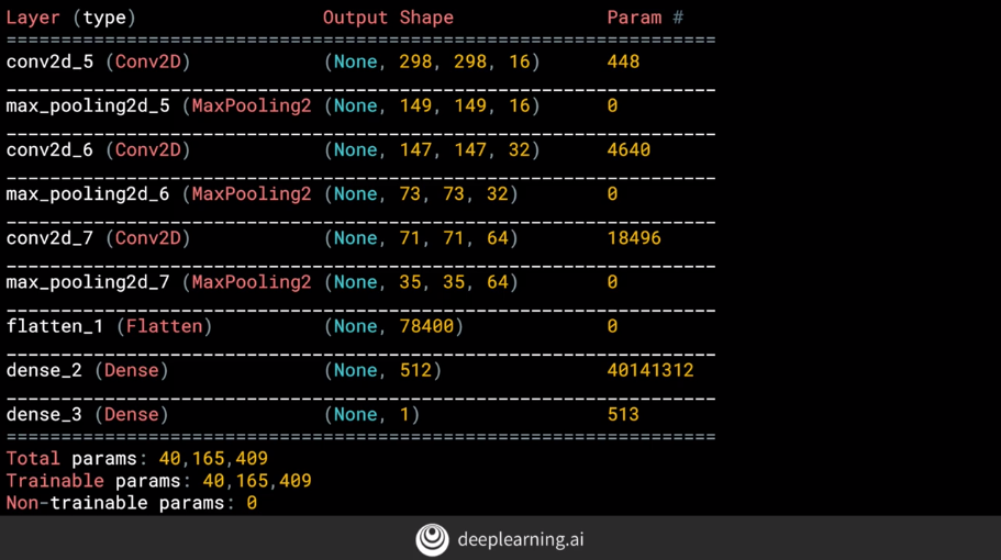
The answers of the questions above are:
- The output of conv layer when padding = 0 and stride = 1 is
(pw-fw+1, ph-fh+1, fn), where pw = picture width, fw = filter width, ph = picture height, fh = filter height, fn = filter number. - Parameters number for the conv2d_5 layer = fw fh fn pc + b = fw fh fn pc + fw fh fn = 3 3 16 3 + 3 3 * 16 = 448, in which b = bias and pc = picture color channels.
Then compile the model:
from tensorflow.keras.optimizers import RMSprop

model.compile(loss='binary_crossentropy',
              optimizer=RMSprop(lr=0.001),
              metrics=['acc'])
Note that we are using a new loss called "binary cross-entropy" and a new optimizer called "PMSprop". Click the corresponding links to check out what they are.
When you use generator, remember to use model.fit_generator(...) as well instead of using model.fit(…).
history = model.fit_generator(
    train_generator,
    steps_per_epoch=8,
    epochs=15,
    validation_data=validation_generator,
    validation_steps=8,
    verbose=2
)
The batch size specified in ImageGenerator for training above is 128, the training folder has 1024 pictures, so need 8 steps per epoch. The batch size specified in ImageGenerator for validation above is 32. The validation folder has 256 images, so we will do 8 steps. And the verbose parameter specifies how much to display while training is going on. With it set to 2, we will get a little less animation hiding the epoch progress.
To classify (either horse or human) of an image, here is the prediction codes:
import numpy as np
from google.colab import files  // colab specific codes for loading images
from keras.preprocessing import image

uploaded = files.upload()

for fn in uploaded.keys():
  # predicting images
  path = '/content/' + fn
  img = image.load_img(path, target_size=(300, 300))
  x = image.img_to_array(img)
  x = np.expand_dims(x, axis=0)

  images = np.vstack([x])
  classes = model.predict(images, batch_size=10)
  print(classes[0])  // sigmoid predicts two values add up to 1
  if classes[0] > 0.5:
    print(fn + " is a human")
  else:
    print(fn + " is a horse")
Note book for week 4: Link without validation dataset and Link without validation dataset
Can also be accessed from Github:
Finally, my thoughts
Should you take this coursera course?
| Yes, if you... | No, if you are... |
|---|---|
| Didn't have any experience of Tensorflow and want to start writing TF codes within 10 minutes. | Familiar with TensorFlow, specifically, used to read TF tutorial, or writing medium size of projects using TF. |
| Want to using TF as a tool and does not really care about how algorithms behind it work. | Want to learn some therotical knowledges on ML. |
| Have no research experience before, try to learn DL/ML to extend knowlegde boundry. | Already doing research in ML/DL (CV, NLP, ASR, etc...), which means you've already used some ML framework even it is not TF. Maybe reading TF tutorial is a better way for you. |
| May already have some experience in some of the ML/DL areas other than CV. This course has a preference to focus on CV, which may help you to learn the CV field. | Already in CV area. |
Be careful! Finishing the course is definitely not the end. You may want/need to dig deeper into the theories behind the metaphors the instructor used to describe concepts. For example, in Quizz 1, "What does a loss function do?" The answer given is "Measures how good the current 'guess' is." But think: What does the Mean Squared Error loss look like? How does it measure how good the current 'guess' is? What does 'guess' means here? These knowledge may help you make decision on NN structure, loss function selection, etc. and most interesting: to feel like Deep Learning is at least a grey box instead of a totally black box. 😎